Exploring Environmental Influences in Cycling
- Introduction
- Building the Dataset
- Feature Engineering
- Exploring the Dataset
- Linear Regression Modeling
- Final Thoughts
1. Introduction
As a hobbyist cycling enthusiast, I am using my bycicle computer, which is a garmin device in my case, for most of my rides. Although so far I'm not super interested in tracking each bit of life, like others do, by wearing a sports watch like the garmin fenix or similar products from other brands, in case of cycling I do enjoy tracking and comparing my rides, to get a sense how i performed or how far I've ridden in the last month. In case of my garmin device, you get access to the garmins platform 'Garmin Connect' where you get dashboards where one can get some insights in the form of nice plots and annotated maps which summarize your individual rides. But without using additional tools these scratch only the surface of what is analytically possible. Aggregation of your ride metrics over a bunch of rides is not possible as far as I know. The analytics remain at the level of an individual session or ride, so to say. It appears interesting to accumulate the data of individual rides into an extensive data set, containing all the rides I did in the last years and look what we can get from that analytically. Mostly my bike journeys can be divided into three categories, which are mountainbiking ('mtb'), road cycling ('road') and 'touring', which summarizes all activities like commuting and bike-packing or bike travel. One may ask what characterizes each of the riding styles in my individual case, since the categories differ in certain attributes, like using different bikes, different riding positions, carrying luggage or not, choice of terrain or length of route, even attitude or motivation when riding may play a role. I'm sure many other relevant variables may come to the readers mind. To track performance related metrics while riding, surely is an established thing nowadays. Many sensors are available for most of the tracking devices (cycling computers or smart watches) used by hobby enthusiasts and professionals. Heart rate sensors and powermeters are probabely the most widely used additional sensors, which promise to give the athlete insight to her riding sessions and provide the possibility to compare her performance to others or her former self. Since I would describe myself as a more mediocre equipped cyclist, I'm relying just on the basic metrics my garmin device is tracking, without using powermeters or heart rate sensors or any additional equipment. Powermeters have definitive advantages over basic tracking, because it allows to get a proxy for the effort put into the riding, which certainly is an interesting quantity for the ambitious rider. Cycling naturally, surely a reason why i love it, happens in the opposite of an controlled environment. Many environmental factors determine the speed and style of riding, like wind speed, wind direction, aerodynamic drag, gradient, and arguably traffic to name just a few important factors. It is hard to evaluate your performance, based merely on your speed, average speed or riding distance.
Goals
With this thoughts in mind, lets summarize the goal for this little project. By accumulating my riding data over the last 2.5 years we'll try to engineer a data set which optimally allows to quantify the influence of environmental factors, like the ones mentioned above, on my riding speed, which serves as the ultimate variable of interest here. The goal is to inference on the influence of environmental factors, which cannot be controlled by the rider, but coped with, and compare these for the three riding styles, mentioned above. For this we will use a simple multiple linear regression to obtain parameter estimates for the environmental influences on riding speed. In difference to machine learnig thechniques where predicition is the goal, here the goal is explanation, like in more classic statistics in the social sciences or economy. We have to come up with a model which can explain to us, not with a model wich on the one hand may more accurately model the underlying data generating process, but on the other hand lacks explainability, because the way the model outputs a probability distribution over a continous range of speed values is hidden in millions of paramters tuned by a gradient descent algorithm. This shall justify the choice of a relatively simple model, which may not fit the data perfectly, but provides easy to interpret results, that may serve our goals. This is to a greater extend an exercise in feature engineering than modeling. The approach can thus be framed as data-centric. Further it must be sayd, that I won't go into too much detail here, since in each aspect of the analysis there are many steps involved, which probabely are not of interest for the reader and would blow up the document to a unacceptable length.
2. Building the Dataset
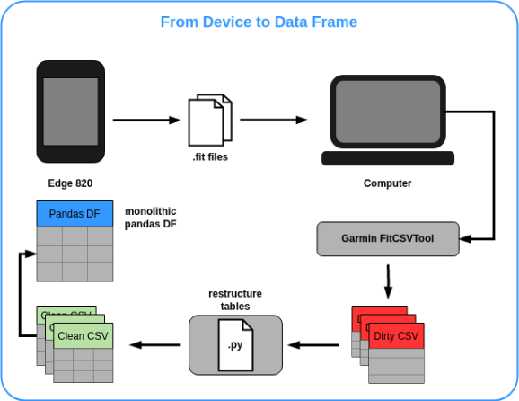
To buid our data set we first have to get the data from the device,
which is a Garmin Edge 820 in my case. We just have to plug it into
the computer and copy the .fit files to a local directory. Garmin
provides a java command line tool, the FitCSVTool
utility, for conveniently converting the data stored in the .fit
files into CSV files. This is nice because it instantly removes some
headaches that you might get when you see files with initially
unknown format that holds the data of interest and you think about
parsing them yourself. The tool delivers CSV files with a bit of a
strange formatting, where information from different granularieties
and categories like device_info,
device_settings and lap are stored into a
single csv. We are mostly interested in the movement profile, which
holds the relevant movement data for each session, like coordinates,
speed and current altitude, which can be found under the category
Message==record. Beyond that the table has a formatting
where the header of the CSV contains 3-tuples of columns that have
elements 'Field k, Value k, Units k', where for each k a specific
variable is stored with its Name, actual Value and the measurement
unit. Further, sometimes more than one session is stored into one
FIT file. These are split into a individual csv tables and we index
them with a local index, so it's easy to keep them appart. To obtain
a data frame, which we can actually work with, some light data
wrangling has to be done, since we like the structure of the CSV to
be classical, with the name of the variables in the header columns
and the corresponding values in the cells. In my case, we obtained
213 CSV files, corresponding to individual sessions, from the FIT
files, including tracked sessions from the last 2,5 years. As it is
often the case with real world data, seldom the data is completely
clean, so while converting the CSV to the appropriate formatting,
some of them are missing relevant data fields like
speed or positional information, which are crucial for
our analyses. We're simply removing these from the data set, which
leaves us with 196 individual sessions CSVs.
3. Feature Engineering
The information we get from the device are:
- Timestamp
- Distance (m)
- Altitude (m)
- Speed (m/s)
- Position Lat/Lon
- Temperature (°C)
For our further analyses we need to convert some of the units used here
for easy later handling when we do some feature engineering. The
positions are stored in semicircles, so we convert them to degree
coordinates for the latitude and longitude values. The timestamp, as you
may read in the well documented
FITCookbook
is encoded in seconds since the Garmin Epoch 1989–12–31T00:00:00 UTC.
Its more handy to convert it into a regularly formatted timestamp which
we can store in a pandas data frame by applying an offset and converting
to the desired format which is YYYY-MM-DD HH:MM:SS. The
positions are converted from semicircles to degrees using a simple
formula:
degrees = semicircles * (180 / 2**31)The speed is converted from m/s to more intuitive km/h. The features we are now engineering are best divided into three categories, which are time-related, weather-related and spatial features.
Time related Features
Here we simply use the timestamps to craft some time related features by applying different resolutions to the time aspect of the data. For each riding session we can compute the elapsed time since start of the ride in seconds. Some informative features regarding the Season of the year and the Weekday, which serve more as descriptive features and won't yield much for inference. Also as time related feature we have subsequently iterated IDs for each data point in each session. It must be noted here that my Garmin Edge 820 provides two modes for data recording which basically set up the sampling intervals at which data is stored while riding. You can choose between 'intelligent' and '1s', where intelligent follows an algorithm that stores data when important parameters are changing, which means that the data is not uniformly sampled over time, and '1s' means strictly recording the data every one second of the ride. I had chosen 'intelligent' for all my rides, so time intervalls between data point are not evenly spaced.
Weather related Features
Now it is getting more interesting. Since the basic data field provide a timestamp along with the corresponding coordinates, we can query a historic weather API to get more relevant data for each place and time of each data point and annotate the data set with this information. Since this is a hobby project we have to restrict our selfes a little bit, because for most weather APIs, the number of queries you can perform in a given timeframe are restricted for the free plans and I don't want to pay for this exploratory hobby project. I've chosen the historical weather API from OpenWeatherMap, which is easy to use, provides enough detailed data, and allows for a sufficient amount of free queries per day. Right now we have over 160.000 data points in our data set. So querying the API for each of the the data points is not feasable at all and also not usefull, because the service won't return weather data temporarly and locally as finely resolved as our riding data is. So we'll stick to the following rule:
# divide session in 10km chunks along the distance
# for each chunk:
# get index of middle data point in the chunk
# get lat/lon for this datapoint
# use the coordinates to call weather API
# propagate the data of each middle point to the whole chunk
Each session get divided into chunks of 10km riding length. For each of the chunks we identify the data point that lays in the middle of the chunk. We will use this data points coordinates and timestamp to query the weather API and retrieve the corresponding data. The data is then propagated to all the data points within the 10km chunk. From the weather API we get:
- humidity (%)
- air pressure (hPa)
- cloudyness (%)
- wind speed (km/h)
- direction of wind (degrees)
- main weather (Clouds/Clear/Rain/Drizzle)
Headwind Intensity
Interesting features, obtained from the Weather API are wind degree and wind speed because it allows to construct a feature that quantifies the amount and intensity of headwind. This is because from our basic data provided positions we may derive the riders bearing at any given point in time from a pair of two coordinates. We then are able to compute the riders bearing relative to the direction the wind is blowing and can obtain a numeric feature which can get multiplied by the wind speed, which directly quantifies the winds intensity to get a combined measure of headwind x wind intensity. The algorithm is as follows: For a pair of subsequent cordinates we compute the bearing of the line connecting those two points in degrees, using the same 360° scale as the wind direction has. We can do this with this little Python function:
# compute the orientation of the line between two coordinates
def get_bearing(from_coords, to_coords):
x1, y1 = from_coords
x2, y2 = to_coords
y = sin(y2-y1) * cos(x2)
x = cos(x1)*sin(x2) - sin(x1)*cos(x2)*cos(y2-y1)
theta = atan2(y, x)
return (theta*180/pi + 360) % 360
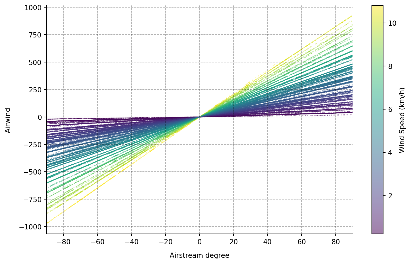
Now we have the direction the rider is heading to in degrees, where 0 or 360 degrees is north, 90 degrees is east, 270 degrees is west and 180 degrees is south, accordingly. Wind direction is defined exactly the other way around where the degree gives the direction from where the wind is blowing, so we have to invert that to get a matching measure. The goal here is to get a measure of 'headwindness' which is called airstream from here on, which has a maximum value of 90 for absolute tailwind and a minimum value of -90 for absolute headwind. Zero is crosswind. This follows the rationale that crosswind has the least influence on our riding speed, while head- and tailwind positively and negatively influences our riding speed. This should make the interpretation of the corresponding regression coefficients pretty straightforward, later. To engineer this, we first compute the bearing of the rider and the wind direction. So we get two angles. From these angles we construct two unit vectors on the unit circle in a standard cartesian two-deimensional vector space as shown in the following figure:
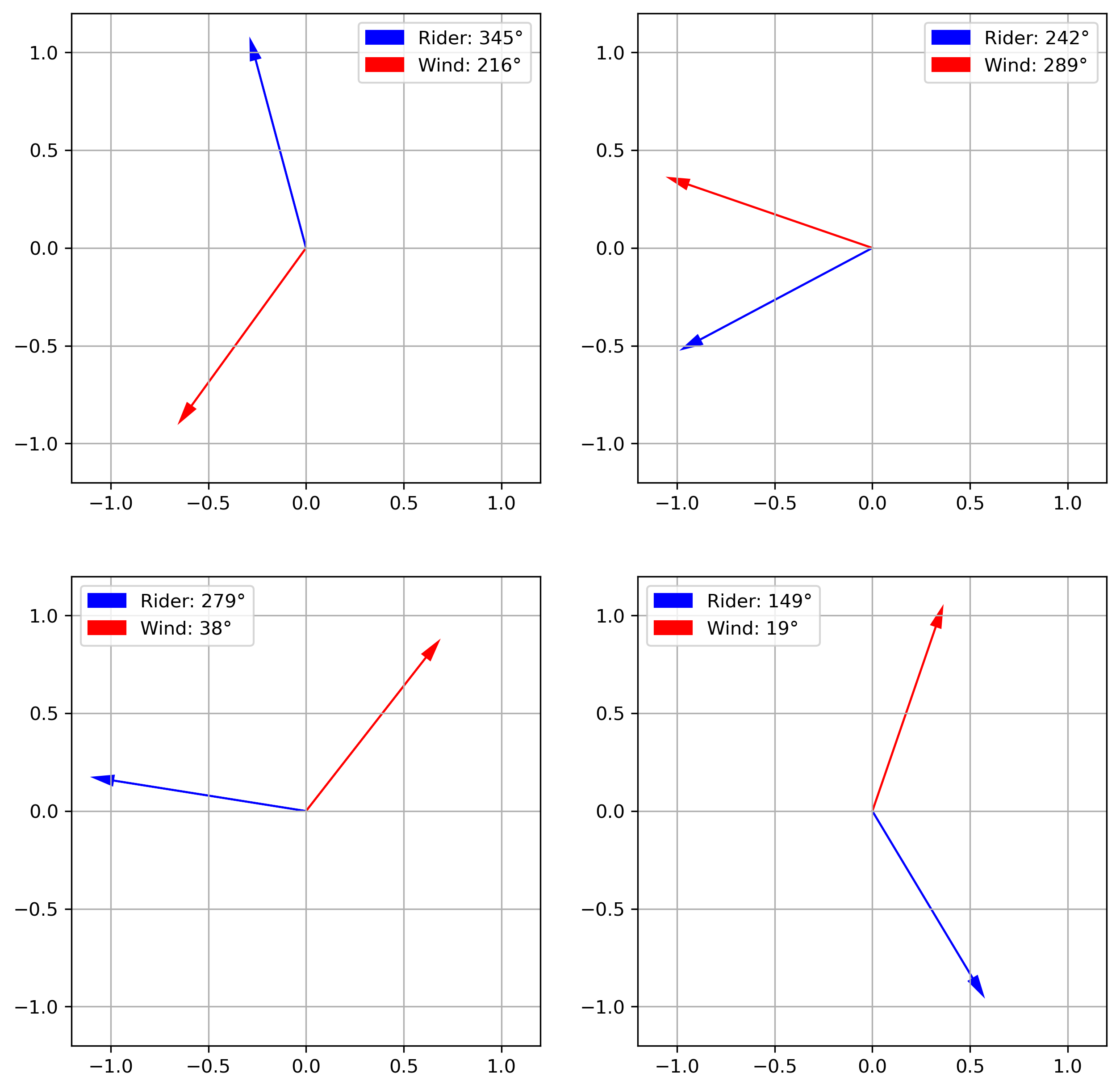
It is now easy to compute the angle between these two vectors. We take the absolute value of the angle between those vectors and subtract it from 90 degrees and there it is, we have the numeric airstream feature with the desired attributes. We can now compute an airstream value for each of the data points in our data set. One problem here, which is worth considering is that the positions yielded by the garmin device are of cause a bit noisy. So for two subsequent positions the riders bearing may not be estimated accurately. This is especcially problematic if the pair of coordinates is in close proximity. See the figure here to understand how this is intended.
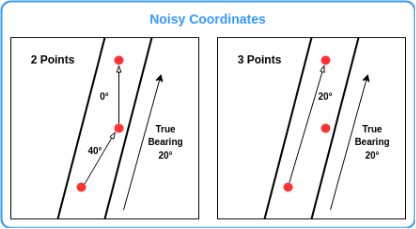
So we try to algorithmically improve this
situation by taking the positions one data point before and one
after the datapoint under consideration to get a pair of coordinates
a bit further from each other and hopefully obtain more stable
approximations of the airstream. It is now just a matter of
multiplying the airstream feature with the wind speed, obtained from
the weather API, to get a feature that numerically represents the
intensity of the headwind for the rider at any given point in space
and time.
Air Density
Another possibly important influential factor is the air density. It's a relevant factor for aerodynamic drag and it's a pure environmental factor. Certainly aerodynamic drag usually plays a bigger role for higher speeds, but as the article Bobridge's Hour points out, it may be worth considering in the equation. Air density can be calculated from the physical quantities we obtained from the weather API (see AirDensityCalculator), which are temperature, air pressure and humidity.
def compute_air_density(temperature, pressure, humidity):
psat = 6.1078*math.pow(10,7.5*temperature/(temperature+237.3))
pv = humidity*psat
pd = pressure-pv
density = (pd*0.0289652 + pv*0.018016)/(8.31446*(273.15+temperature))
return density
Spatial Features
Usually it is inevitable that my rides passing some sort of urban area, where we have to deal with traffic, and generally more obstacles, which certainly has an influence on the riding speed. Thus, it would be informative to know for each data point if the coordinate is in a town, village or other urban area. Further, the kind of road or path we're riding would be an informative feature, too. If you have experience in riding road bikes, I'm sure this makes intuitively sense to you. Riding on the smoothest asphalt is in most cases optimal for the narrow road tires, ridden with relatively high tire pressures, while approaching bumpy paths makes you neccessarily go slower. My approach to obtain both of these information is again to query external services to get the relevant data.
Urban/Rural Labels
For the urban area feature the approach is to use map images and computer Vision techniques to obtain a binary label, which tells if the coordinate is in urban or rural area. The construction of this classifier will get explained in another post on this website, but the general idea is to use the GoogleMaps API to construct a training data set of map images from germany (where most of my rides take place), which is used to train a simple CNN (Convolutional Neural Network) classifier. The classifier may then be used to classify the map images, which are queried from the API for each data point in the data set.
Acquisition of OSM Tags
The road type features are obtained by using data from OpenStreetMap. OSM provides detailed tags for a huge amount of roads and paths. These are basically key-value-pairs, where the values hold the information we're interested in. Under these tags, of special interest are the 'highway', 'surface' and 'smoothness' tags. The highway tag encodes information about the importance of the road, like motorways, primary roads or paths. The surface yields information roughly about the material the road is made of, like asphalt, gravel or cobblestone. The smoothness tag gives ordered information about the quality of the road, like 'good', 'intermediate' or 'bad'. It's not totally trivial to get these information, so in order to keep the length of this article within limits, the process of retrieving these information will be explained in the corresponding article on this website. But as a general overview, we download an OSM europe extract from Geofabrik, build a local SQLite database from it and use the SpatiaLite extension to build a spatial index for fast spatial queries. The procedure here is to build a bounding box around the coordinates of each data point in the data set. This bounding box is used with the spatial index and helps to obtain osm nodes, which belong to osm ways, without waiting for hours for the query to complete. For each coordinate we get multiple ways within the bounding box, so we compute for each of the ways the distance to the query coordinate and choose the closest way. From this we get the tag information mentioned above. This is done for alle the around 150.000 data points which are in the data set at this point. After obtaining the tags, for 'highway' and 'surface' we group the possible variables into broader categories, to reduce the number of possible values. These two are nominal variables, which will become one-hot-encoded later, and having 38 different values for the highway tag would intoduce 37 additional columns to the data set and blow up the dimensionality of the feature space in an undesired amount. So for 'highway' we're left with the possible values:
- path
- residential
- secondary
- track
- tertiary
- trunk
- primary
- motorway
- cycleway
- construction
- unclassified
- cobblestone
- unpaved
- paved
We have to solve another classic problem of real world data, which is missing data. While we have the highway tags for 100% of the data points, we get the surface tags for just above 89% of the coordinates, and the smoothness tags for circa 71% of the data points. Since our analytical approach is linear regression, we have to deal with this problem, since missing data cannot be used with this technique. To solve this, the missing data is imputed with the help of a random forest classifier. The classifier is trained on the data points where the data isn't missing and predicts values for the data points where the data is missing. This is a reasonable approach for multiple imputation, because it takes into account all the existing information and doesn't introduce that much bias into the data set as simple single variable imputation techniques would cetrainly do.
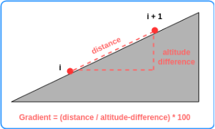
Computing the Gradient
Since we already have the distance ridden for each data point, and also
computed the difference in altitude between two subsequent data points,
we can easily compute the gradient, as shown in the figure. It just
quantifies the amount of elevation for a given amount of distance
ridden. The practical relevance of this feature should be clear to
everyone who ever rode a bike.
Preparation for linear Regression
Now we have all the features in place. Some outliers are
identified, namely a session that was a car ride as well as one that
was a hiking trip. We don't want them in the data set, so they're
simply excluded. After the gradient computations it turns out that
there are a few data points with unreasonable high gradients above
+/- 20%. Since these are just 0.45% of the whole data set, they get
removed as well. We further drop rows where speed is zero, since
they don't be of much value for the analysis. There are also a few
sessions which most likely were testing session and/or sessions with
broken recording, that have a total distance of less than 5km. They
are also excluded from the data set. This leaves us with 152.726 data points.
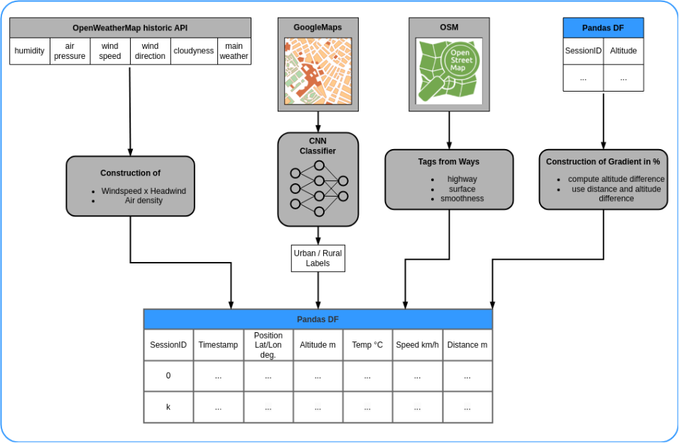
To give a brief overview over the feature engineering performed as described above,
the following figure summarizes the features we engineered:
4. Exploring the data set
Before we come to the modeling part, let's briefly explore the data set, and show some numbers and distributions, which may come in handy for the interpretation of the results later. For the sake of brevity, again, we wont go into too much detail here. As an first overview, we can see that I recorded 26 mountainbike rides, 83 road rides and 68 touring rides. The most common sessions are road bike sessions, and mountainbike rides are the least. As expected, the average speed is highest for road rides, followed by touring rides and mtb rides are slowest. The relatively low average distance for touring rides is due to the fact that these rides are mixed up with commutes, which are mostly of short distance. In general, bikepacking rides tend to be longer, as you would expect:
| session_type | count | avg_speed | avg_distance |
| mtb | 26 | 22.89 | 24.28 |
| road | 83 | 29.68 | 26.99 |
| touring | 68 | 23.09 | 19.81 |
The descriptive results here, can be seen as a sanity check for the
building process of the data set. If our expectations wouldn't be met,
there would be a good reason to go back and check the data wrangling.
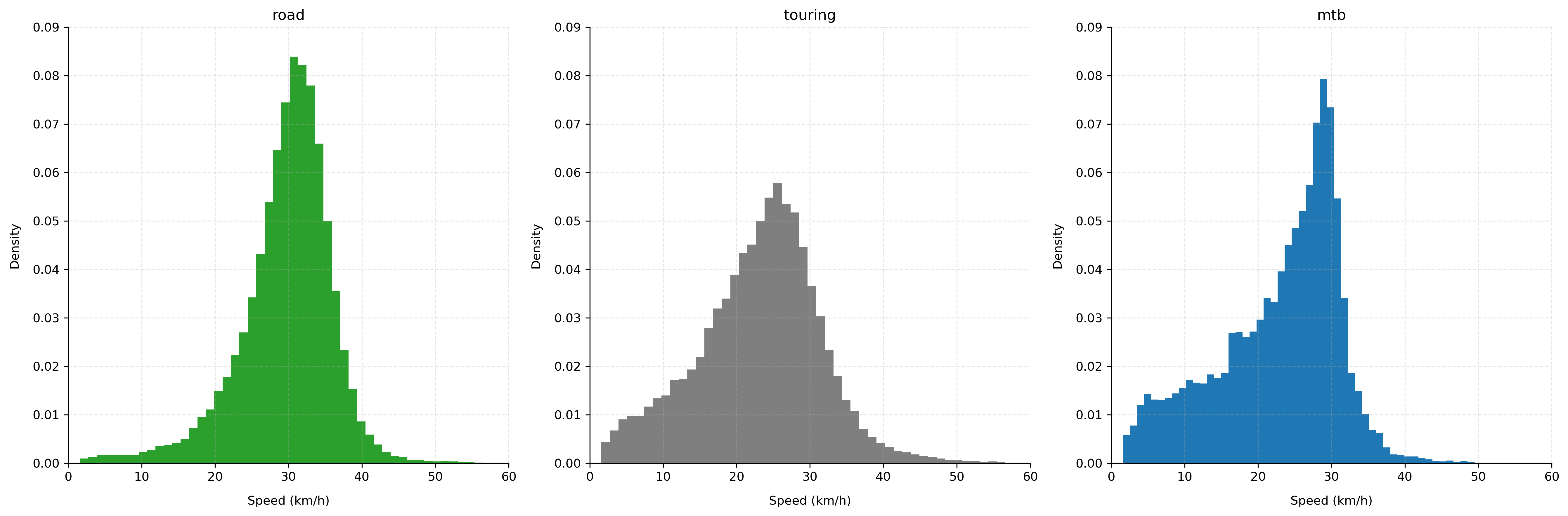
Let's look at our main variable of interest now, which is the riding speed,
and compare the distributions for the three riding styles:
We constructed features that are expected to have a real influence on
our dependet variable (DV, speed). So its allways a good idea to look at
corresponding scatterplots to see if there is visual indication for a
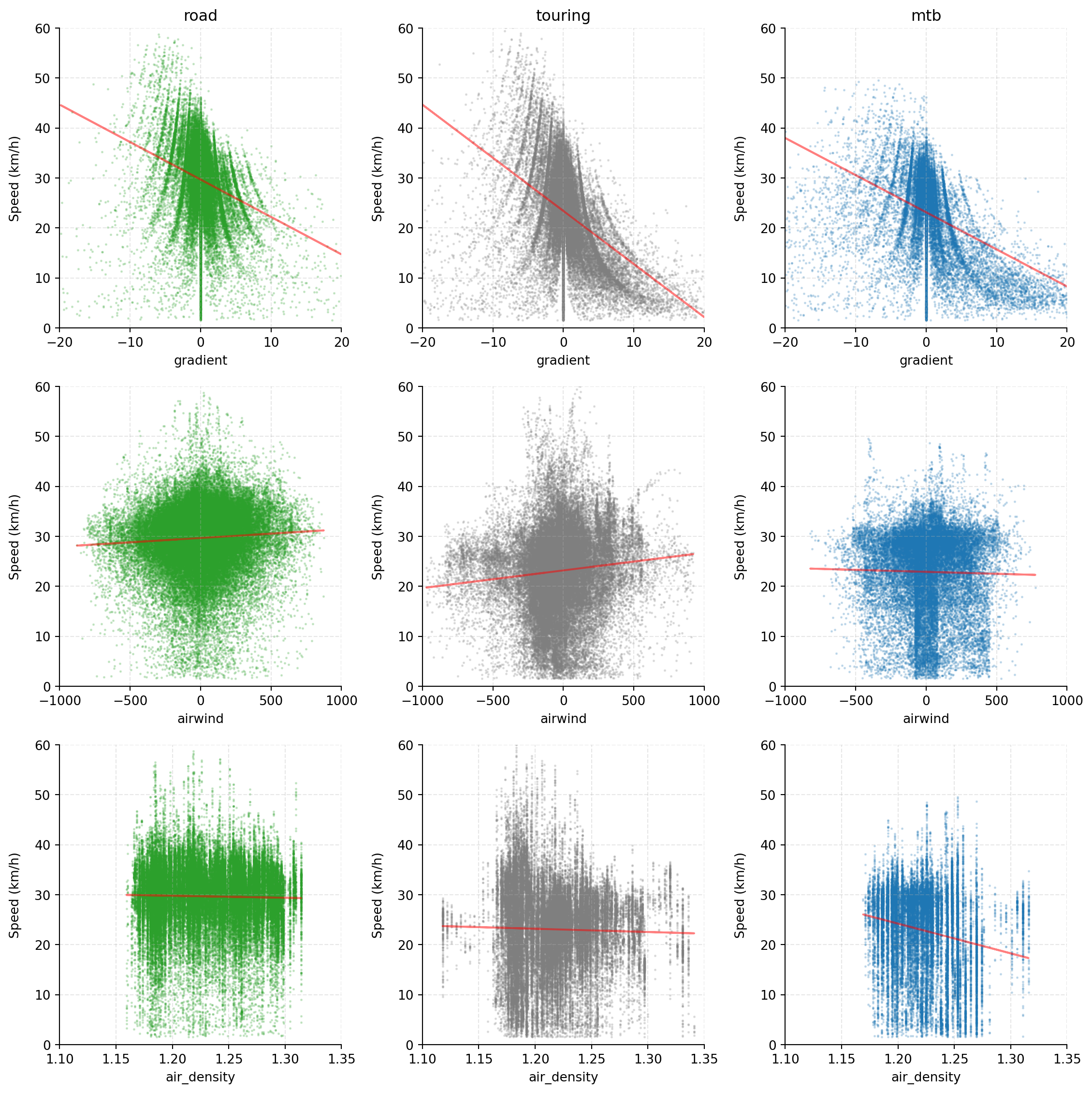
relevant relationship between these features and the DV. Lets look at our
self assembled numeric features and the DV:
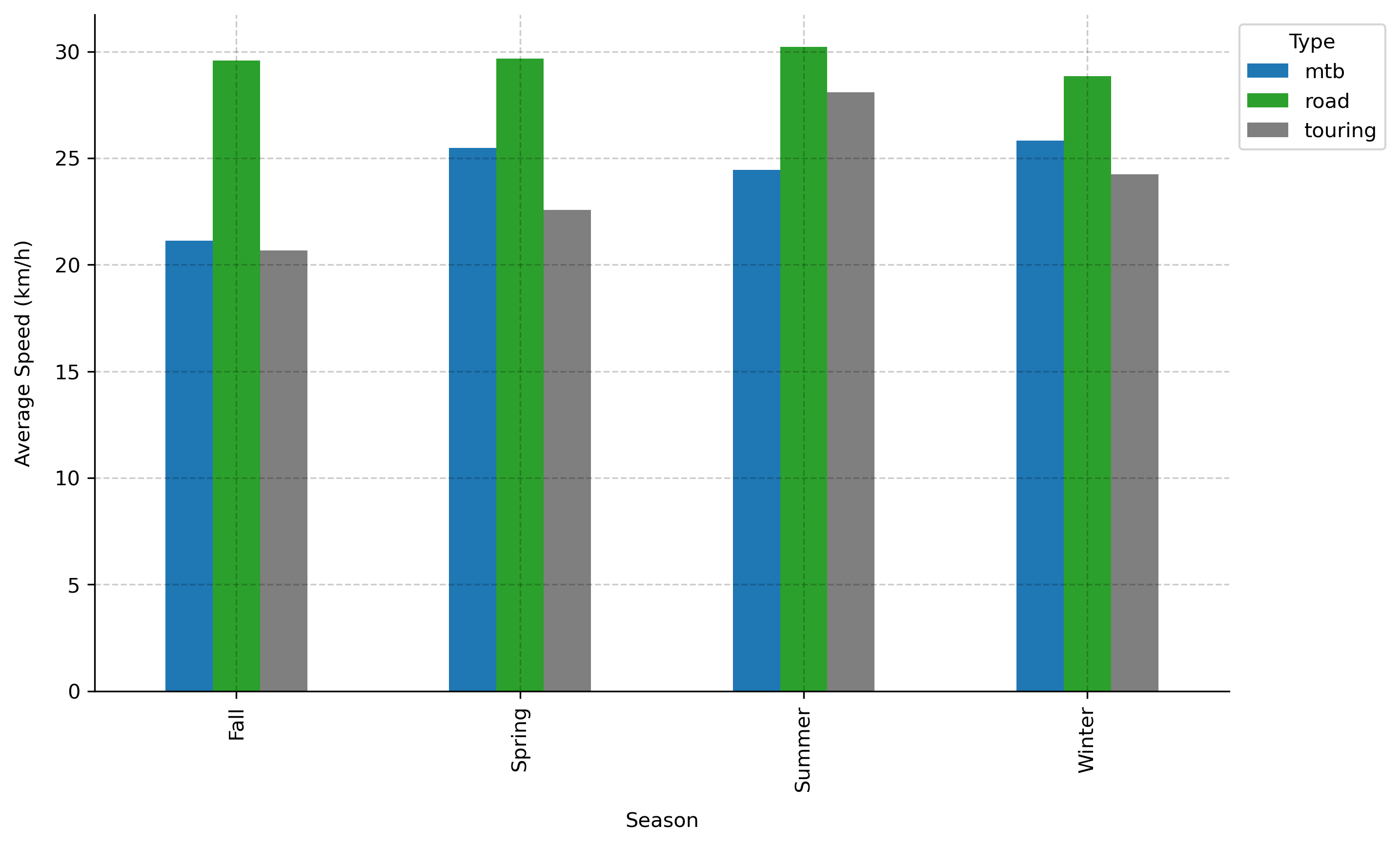
And just for fun, let's check my average speeds per season of the year and
riding style:
5. Linear Regression Modeling
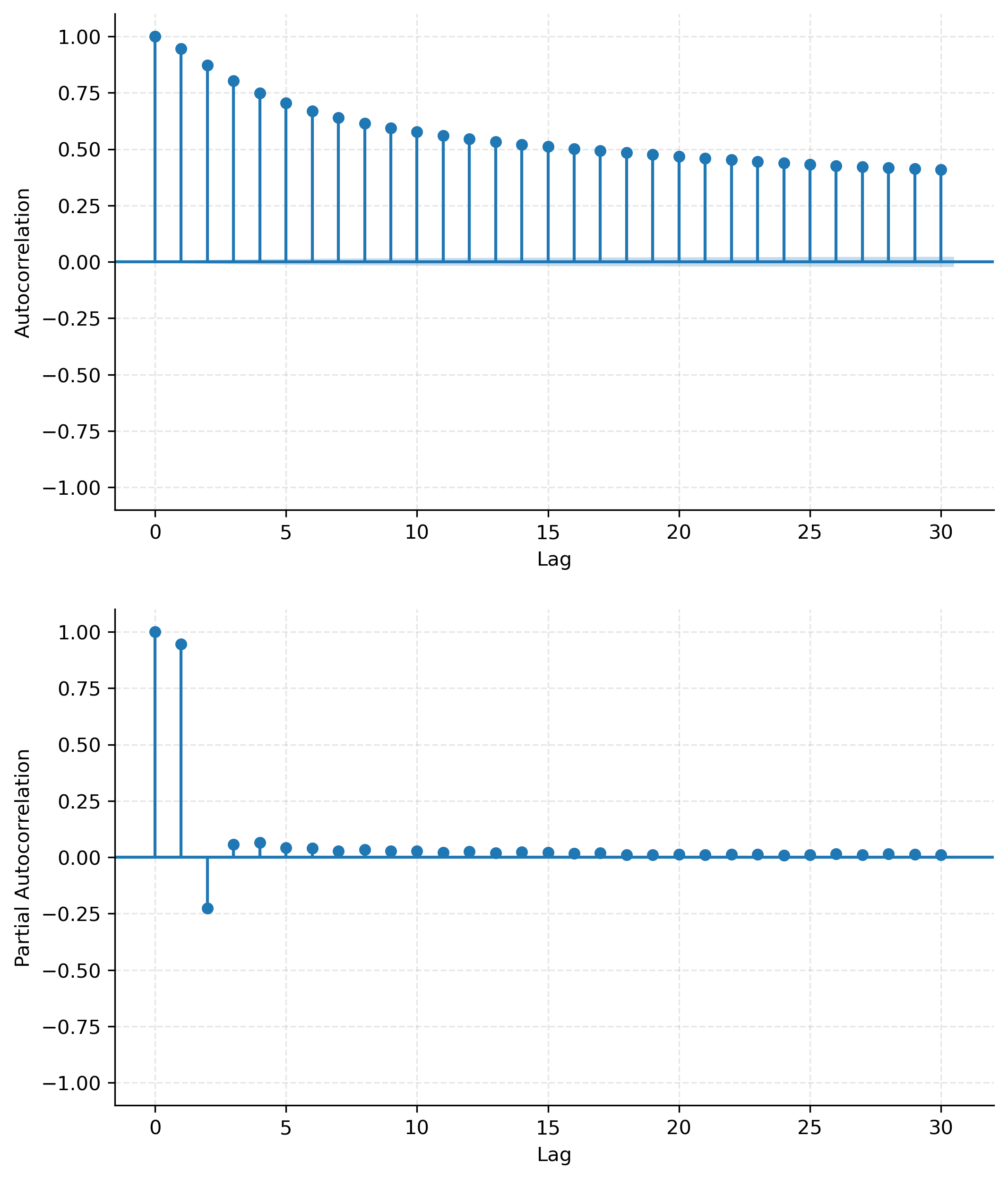
As pointed out earlier, we're using a rather simple linear regression model, to model the relationship between the riding speed and the features we engineered. As a quick reminder or for those who are not too familiar with linear regression, the idea is to model the dependent variable (speed in this case) as a linear combination of the independent variables (the features we obtained and the ones we engineered), where a residual term captures all the unexplained variance, which our model cannot account for. There model is linear in its parameters. There are several assumptions that should be met for a OLS (ordenary least squares) regression model to yield unbiased estimates of the parameters we're interested in. We can't analyze all of them here, but the most important one is the assumption of iid (independent and identically distributed) samples. This is a crucial one here, because we have good reasons to suspect that this is not met by our data, as we show in the next section with the help of autocorrelation plots.
Autocorrelation structure
Our data has obviously a strong temporal structure, since the data
points are ordered by time. The individual sessions are
multi-dimensional time series. This means, that our speed at a specific
point in time is highly correlated with one or more data points before.
Thus the iid assumption is not met. Generally this is called
autocorrelation, and we have to account for that in our modeling
choices. The severity of autocorrelation can be measured with the help
of the autocorrelation function (ACF), which we plot to see how strong
the correlation is for different lags.
Model Choice
We have to deal with this autocorrelation structure when choosing a model. Here we have several choices, like ARIMA models, which are specific for time series data or linear mixed effects models, which are able to account for the grouped structure of our data. It's considered grouped because we have individual riding sessions concatenated in our data set and data points inside of these sessions are highly correlated, while outside of the sessions they most likely are not. Each of these models come with their own challenges and caveats. Further we have sessions of variable length, that is different number of data points. Also the temporal spacing is not even between the data points, since my Garmin device recorded the data with unevenly spaced intervals in the 'intelligent' mode. The main point here is that we're not particularly interested in the temporal structure of the data, but in the influence of the features on the speed. Still, we have to account for the autocorrelation to obtain estimates which we can trust. The problem with autocorrelation in OLS regression is not that the point estimates are wrong, but the standard errors are underestimated, when the autocorrelation is not accounted for. This leads to wrong conclusions about the significance of the estimates. We'll approach this problem by using OLS regression and correct the standard errors with the help of covariance matrix estimators that account for the autocorrelation, and cluster robust standard errors. The clustering here is done by the session ID, which is the grouping variable. This appears to be a feasible approach, where we don't loose the interpretability of the results, but still get unbiased estimates, while at the same time beeing quite fast and simple.
We will first run a baseline model where we're modeling just with the basic set of variables that we obtained from the Garmin device. They won't be very informative for our model, but it's allways good to have a reference point. Then we will add our crafted features and run the model again to see how much variance in the DV we can explain with them. As mentioned before we're modeling the riding styles seperately, and compare the results for individual types.
Results
Let's now have a look at the results for the regressions. We'll report parameter estimates, standard errors and p-values at the 0.05 level for each feature in the model and for each riding style. We'll also report the R² values for each model to see how much variance of the dependent variable our model can explain, and also AIC and BIC scores for model comparison. For those who are unfamiliar with linear regression estimates, the rationale for interpretation of the results can briefly be summarized as follows: Each parameter estimate tells us how much the dependent variable changes, when the independent variable changes by one unit, while all other variables are held constant. So, for example, if our paramter estimate for altitude is -0.05, this means that our riding speed drops by 0.05 km/h for every 1m increase in altitude, if all other variables stay the same. The intercept in the tables is different to interpret, since the intercept is the estimated value of the dependent variable, when all independent variables are zero. Since we're centering our metric variables, it represents the average speed of the condition at the average of the independent variables (the features), and at the zeros of the categorial features. The standard error tells us how much the estimate is uncertain, and the p-value tells us if the estimate is significantly different from zero. If the p-value is below a certain threshold, usually 0.05, we can reject the null hypothesis that the parameter estimate is zero. This means that the feature has a significant influence on the dependent variable.
Baseline
Parameter Estimates
| intercept | distance | temperature | altitude | ||
| mtb | parameter | 22.89491 | 5e-05 | 0.04722 | -0.0393 |
| mtb | std_err | 0.35804 | 3e-05 | 0.07765 | 0.00421 |
| mtb | pvalue | 0.0** | 0.1531 | 0.54855 | 0.0** |
| touring | parameter | 23.0858 | 0.0 | 0.12561 | -0.01386 |
| touring | std_err | 0.4582 | 1e-05 | 0.0682 | 0.00448 |
| touring | pvalue | 0.0** | 0.89145 | 0.06993 | 0.00286** |
| road | parameter | 29.67802 | -0.0 | 0.01713 | -0.00155 |
| road | std_err | 0.19744 | 2e-05 | 0.0273 | 0.00468 |
| road | pvalue | 0.0** | 0.97478 | 0.53213 | 0.74134 |
At our baseline we see that we cant explain much with the model built upon the basic features. The double-star notation at the p-values denotes which parameter estimates differ significantly from zero at the alpha level of 0.05. Altitude here, is the only feature which as any significant influence on the speed for mtb and touring sessions. For road sessions none of the features are significant. For reference we report the model fit statistics here:
Model Fit
| R² | AIC | BIC | |
| mtb | 0.177 | 194543.4055 | 194576.4108 |
| touring | 0.048 | 361944.8969 | 361980.2882 |
| road | 0.000 | 476598.7006 | 476635.4926 |
It's woth noting that we have a relatively high R² for the mtb sessions, where altitude appears to be quite informative for the model in predicting the riding speed from it. This may be due to the fact, that my mtb sessions usually start in the valley, on streets and good quality paths, where I can ride with higher speeds as compared to the gnarly and bumpy paths up on the mountain. So this is an issue of uncontrolled covariates, which may lead to false conclusions. Let's expect, that this relation won't be significant once we start to control for the type of street and surface we're riding. Probably we may observe this behavior in the full model.
Simple Model
Now we're using some of the crafted features and see how this affects our model. We're adding the gradient, airwind and air density. At the same time we drop the naive features frome the baseline model.
Parameter Estimates
| intercept | gradient | airwind | air_pressure | ||
| mtb | parameter | 22.89491 | -0.73488 | 0.00013 | -0.23377 |
| mtb | std_err | 0.70668 | 0.07081 | 0.00103 | 0.10328 |
| mtb | pvalue | 0.0** | 0.0** | 0.90093 | 0.03254** |
| touring | parameter | 23.0858 | -1.05501 | 0.00308 | -0.13807 |
| touring | std_err | 0.46073 | 0.08381 | 0.00144 | 0.05547 |
| touring | pvalue | 0.0** | 0.0** | 0.03545** | 0.0153** |
| road | parameter | 29.67802 | -0.75107 | 0.00179 | -0.00741 |
| road | std_err | 0.19887 | 0.06041 | 0.00033 | 0.02065 |
| road | pvalue | 0.0** | 0.0** | 0.0** | 0.72042 |
Model Fit
| R² | AIC | BIC | |
| mtb | 0.203 | 193626.8567 | 193659.8620 |
| touring | 0.201 | 352901.7200 | 352937.1112 |
| road | 0.063 | 471916.4565 | 471953.2485 |
Over all we're doing way betetr here, as the fit statistics show quite an improvement in R² for mtb and touring, but just a little for road sessions. The gradient parameter is significant for all riding styles, while the size of the change in speed for each percent of gradient increase is the highest for touring and the lowest for mtb. Since my touring sessions are almost always with luggage, therefore a higher overall system weight, this makes sense. For each percent of gradient increase my speed drops by around 1 km/h in touring sessions. The influence of headwind appears to be the highest in touring sessions, which also makes sense, because of the most upright riding positions as well as the added aerodynamic resistance, which comes with attatching bags to the bike. Interestingly for the mtb sessions, the headwind intensity doesn't seem to play a role. This could be due to the fact that my mtb rides are for the most part in the woods, where wind doesn't play a major role. The air pressure estimates are differing significantly from zero for mtb and touring sessions, but not for road sessions. It's quite hard to interpret that. Since the headwind obviously plays a role in road bike sessions, one cannot conclude that it's probably the riding position and the aerodynamics of the road bike, that causes this difference. The only reason that appears to make sense to me is that my road sessions are mostly on flat terrain and don't contain muchh altitude changes, which would influence the air density towards more variation for each ride.
Full Model
Now let's compute the full model, where we add the features from the OSM tags and the urban/rural classifier, as well as keeping some features from the baseline model. Let's recall here that the levels of the variables 'highway' and 'surface' were one-hot-encoded, so each level turned into an own 1/0-encoded variable (accordingly they're denoted by the prefixes 'h' and 's'). The reference categories, which are 'trunk' for 'highway' and 'cobblestone' for 'surface' do therefore not appear in the model. So the intercepts represent the average speed for these two values. For the google maps urban/rural classifier, the reference is 0 which means 'rural'.
Parameter Estimates
| intercept | gradient | airwind | temperature | humidity | air_pressure | altitude | smoothness | ||
| mtb | parameter | 14.43474 | -0.70697 | 0.0001 | 0.01817 | -0.02251 | -0.03168 | -0.02888 | -1.30163 |
| mtb | std_err | 2.94851 | 0.05852 | 0.00086 | 0.07215 | 0.02631 | 0.04072 | 0.00551 | 0.14381 |
| mtb | pvalue | 5e-05** | 0.0** | 0.90977 | 0.8032 | 0.40023 | 0.4438 | 2e-05** | 0.0** |
| touring | parameter | 9.67449 | -0.9884 | 0.00227 | 0.14051 | 0.033 | -0.12503 | -0.01492 | -0.32063 |
| touring | std_err | 2.15417 | 0.0922 | 0.00102 | 0.05459 | 0.02419 | 0.0472 | 0.00275 | 0.24958 |
| touring | pvalue | 3e-05** | 0.0** | 0.02977** | 0.01227** | 0.17719 | 0.01006** | 0.0** | 0.20332 |
| road | parameter | 19.54356 | -0.72846 | 0.00186 | 0.0285 | 0.00109 | -0.0043 | -0.00502 | -1.29351 |
| road | std_err | 1.84561 | 0.05477 | 0.00035 | 0.02232 | 0.01109 | 0.0224 | 0.00437 | 0.11318 |
| road | pvalue | 0.0** | 0.0** | 0.0** | 0.20512 | 0.92202 | 0.8484 | 0.25415 | 0.0** |
| urban | h_path | h_residential | h_secondary | h_track | h_unclassified | h_cycleway | h_tertiary | ||
| mtb | parameter | -0.49947 | 6.54533 | 5.48698 | 3.16559 | 7.41818 | 8.34252 | 8.24062 | 6.49517 |
| mtb | std_err | 0.32478 | 2.52624 | 2.62562 | 3.18739 | 2.6667 | 2.91296 | 2.57646 | 2.99285 |
| mtb | pvalue | 0.13664 | 0.01575** | 0.04697** | 0.33015 | 0.01013** | 0.00835** | 0.00373** | 0.03969** |
| touring | parameter | -2.86552 | 11.56197 | 10.35781 | 13.39754 | 12.28268 | 13.7475 | 11.80971 | 12.79904 |
| touring | std_err | 0.33096 | 2.01898 | 2.03991 | 2.11881 | 2.04394 | 2.08811 | 2.03372 | 2.09752 |
| touring | pvalue | 0.0** | 0.0** | 0.0** | 0.0** | 0.0** | 0.0** | 0.0** | 0.0** |
| road | parameter | -2.79888 | 8.5205 | 8.91621 | 8.57 | 9.00102 | 11.8142 | 9.06659 | 7.50878 |
| road | std_err | 0.19837 | 1.80185 | 1.8482 | 1.81524 | 1.8319 | 1.92411 | 1.85327 | 1.88462 |
| road | pvalue | 0.0** | 1e-05** | 1e-05** | 1e-05** | 0.0** | 0.0** | 0.0** | 0.00015** |
| h_primary | h_motorway | h_construction | s_unpaved | s_paved | ||
| mtb | parameter | -2.74731 | -4.59479 | -12.26232 | 1.81874 | 2.44259 |
| mtb | std_err | 2.96697 | 2.78834 | 5.37375 | 1.20275 | 1.1123 |
| mtb | pvalue | 0.36332 | 0.11189 | 0.03127** | 0.14303 | 0.03759** |
| touring | parameter | 8.78758 | 10.7864 | 11.99029 | -0.51931 | 3.48077 |
| touring | std_err | 2.04882 | 2.38803 | 2.26161 | 0.83904 | 0.60146 |
| touring | pvalue | 6e-05** | 3e-05** | 0.0** | 0.53806 | 0.0** |
| road | parameter | 5.96914 | 5.00533 | 4.07094 | 1.34196 | 2.77656 |
| road | std_err | 2.88734 | 2.28063 | 3.32736 | 0.72814 | 0.70465 |
| road | pvalue | 0.04186** | 0.03101** | 0.22465 | 0.06894 | 0.00017** |
Model Fit
| R² | AIC | BIC | |
| mtb | 0.358 | 187516.3516 | 187689.6294 |
| touring | 0.319 | 344694.1461 | 344879.9499 |
| road | 0.204 | 459986.9441 | 460180.1023 |
By looking at the model fits, we can explain a lot more variance with the full model. For the mtb model we're able to explain 35% of the total variance in speed just by considering environmental factors. For the road bike sessions, again we can explain the least amount of variance, bit still we did a huge step from our simple model with just 3 predictors. Some of the results we observed with the simple model still hold in the full model, while other changed. The gradient is still significant for all riding styles, and has a considerably high influence on the speed. The headwind intensity ('airwind') is relevant for road and touring, but not for mtb sessions. In difference to the simple model the air density isn't significant for mtb anymore, while the altitude is still significant, but with a lower parameter estimate. The smoothness of the surface shows a quite high influence on the speed for mtb and road bike sessions, while appears not to affect the touring sessions. This may be due to the overall lower riding speed when commuting or travelling, where I usually dont push that hard, like I do when riding mtb or road. This results in a smaller need to reduce my riding speed when approachin roads or paths of bad quality. As one would expect, for all riding styles, we're going faster on paved roads than on unpaved roads and cobblestone. The google maps urban/rural classifier seems also to account for a good portion of the variance in the speed. While the estimate isn't significant for mtb riding, it clearly makes a difference for touring and road bike sessions.
6. Final Thoughts
We managed to explain a good amount of variance in the riding speed with the full models, which is awesome. Most of the results are somewhat intuitive but certainly the interpretation and reasoning about why a certain feature has an influence on speed in which case is challenging as one needs some background information about my riding habits. And still there remains quite a bit uncertainty in these interpretations. It is important to mention that the feature engineering certainly introduces some bias into the whole analysis. Some of the features are quite coarse, like all the features derived from the weather data, which sampling resolution is determined by the density and availability of weather stations, which the report to the weather API that we used. The CNN Classifier itself is not totaly accurate, with a reported testing accuracy of around 95%, there will be some missclassified samples. Also the clustering of the OSM tag values is somewhat abritrary. We did data imputation for the missing OSM tags, which may introduce some bias, too. Let's also consider here that there are indications that the linear model won't provide the best fit, as we can see from the scatterplots. There, for instance, you can observe that the gradient has clearly not a linear relationship to speed. This may be also true for other features. But for the sake of simplicity and interpretability we sticked to the linear model of speed. It is a reasonable assumption that even using non-linear transformations of the features, like in polynomial regression would lead to a better model fit to the data. In this regard it is still surprising that we could explain that much variance with the linear model in some cases. Of cause it would now be of much interest to have powermeter measures to have a proxy for the effort that is put into the riding. It would be interesting to see how well we could fit the data with our model, if we had this information, possibly allowing to make mor reliable conclusions about the influence of environmental features versus features that stem from the riders abilities or efforts. Moreover we could go way harder into the feature engineering, by construction more relevant features from the OSM data, like distance to the next crossroads or traffic light, or leveraging more of the possible tags, since there are much more available for a given way, but with lower coverage in the OSM data itself. The approach of using composite google maps sattelite images could also be expanded, to build a more diverse classifier, that could also distinguish between beeing in a forest or on a field, and that alike. Another fruitful source of variance is probably the gear one is using, which isn't really captured at all in this analysis. Sometimes I change things at my bikes, like swapping cranks or handlebars or even the wheelset. Things like that are not considered at all in the current model, but would certainly be intzeresting points to take into account when building upon this analysis in future work.