Building a CNN urbanity Classifier with Map Images
1. Introduction
For my Cycling Data Analysis project, I had a decent amount of locations, given as lon/lat coordinates. For these coordinates I wanted to know if each individual location is in an urban or rural area. When distinguishing between urban and rural areas, this differentiation is made with the context of the problem in mind, which is that each location is a point of a cycling route, at a specific time. So for the locations it's not about beeing inside a specific administrative boundary, it's more about beeing close to any kind of settlement or beeing in the periphery, where you won't have much traffic, cross roads, traffic lights, pedestrians or other urban obstacles. Solving this problem, is not easily done with a simple rule based system or by checking with a reverse geocoder if the location is inside a city boundary. Cities sometimes contain sparser areas, probabely more towards the outer parts. We'd need the administrative boundaries in form of a shapefile polygon, or something like this, to reliably check if a certain coordinate is within a city, town or village.
For my master's thesis, I worked with remote sensing data, so, for me, it's a straightfoward idea to treat the problem of classifying the locations as urban or rural as a supervised learning problem for a neural network operating on map images. If you look at google maps images of these areas I am pretty sure it's fairly easy for you to distinguish between these areas. I am quite sure a neural network clasifier can do this as well, since there are clear regular patterns and structures, formed by streets and buildings in urban areas, which are not present in rural areas.
So this little article is about building such a classifier, with the common steps of data set acquisition, including getting the ground truth labels, that are neccessary for supervised learning, choosing a model architecture, training the model and lastly evaluation of the models performance for the given task.
2. Training Data Set Construction
Map images are a data source that is widely available through web services like openstreetmap (OSM) or google maps, which makes it pretty straightfoward to collect a suitable data set for the classification task outlined above. The main questions here are cost, parametrization and map image type. Usually the user may choose from different map layers like satellite, terrain or more abstract street maps. We like to choose a style where enough information is present for the classifier to distinguish certain features. Further, we like to parametrize our procedure of querying the map images, so that we have controlable consistency in the attributes of the images, like the zoom, resolution and, of cause, the location of the map image. Before we get to building the data set, here is a brief overview of the main python libraries we will use throughout this project:
| Library | Function |
| requests | calling API endpoints and retrieving map images |
| geopandas | spatial functions for retrieving location for the map images |
| shapely | just for the Point object, which we use together with geopandas |
| tensorflow/keras | neural network training and inference |
| sklearn | conveniently computing evaluation metrics for the trained classifier |
The main environment for this project is based on python 3.12, with the classic stack of numpy, pandas, and matplotlib.
Where to get what images?
I decided to go with the google maps static map images API, which provides all the features we need. One needs a google account for this and you have to register for an API key by creating a project in the google cloud console. Google provides 300$ of free credits for new users and 200$ free credits every month, which should be enough for the purpose of this project. As this is just a side-quest of my hobby cycling analysis project, I really don't want to pay anything for the data. After obtaining the API key, we're ready to get the map images, by making calls to the corresponding API endpoint with the parameters of zoom level, image size, center location of the map images in lat and lon coordinates, the type of map and the API key, of cause. We simply call the API with requests and get the images bytes:
r = requests.get(f"https://maps.googleapis.com/maps/api/staticmap?center={lat},{lon}&zoom={zoom}&size={height}x{width}&maptype={MAPTPYE}&style=feature:all|element:labels|visibility:off&key={GMAPS_API_KEY}")
img = r.content
stream = BytesIO(img)
with Image.open(stream).convert("RGBA") as image:
  img_array = np.array(image)

# store the image array to disk here
The style parameter
style=feature:all|element:labels|visibility:off
controls the presence of annotations like street names, which we don't want to
have in our images, since we don't want the classifier to be fooled by the
presence of text or other cues, that don't belong to the features we want to
classify. We have four options for the map types, which are rendered below:
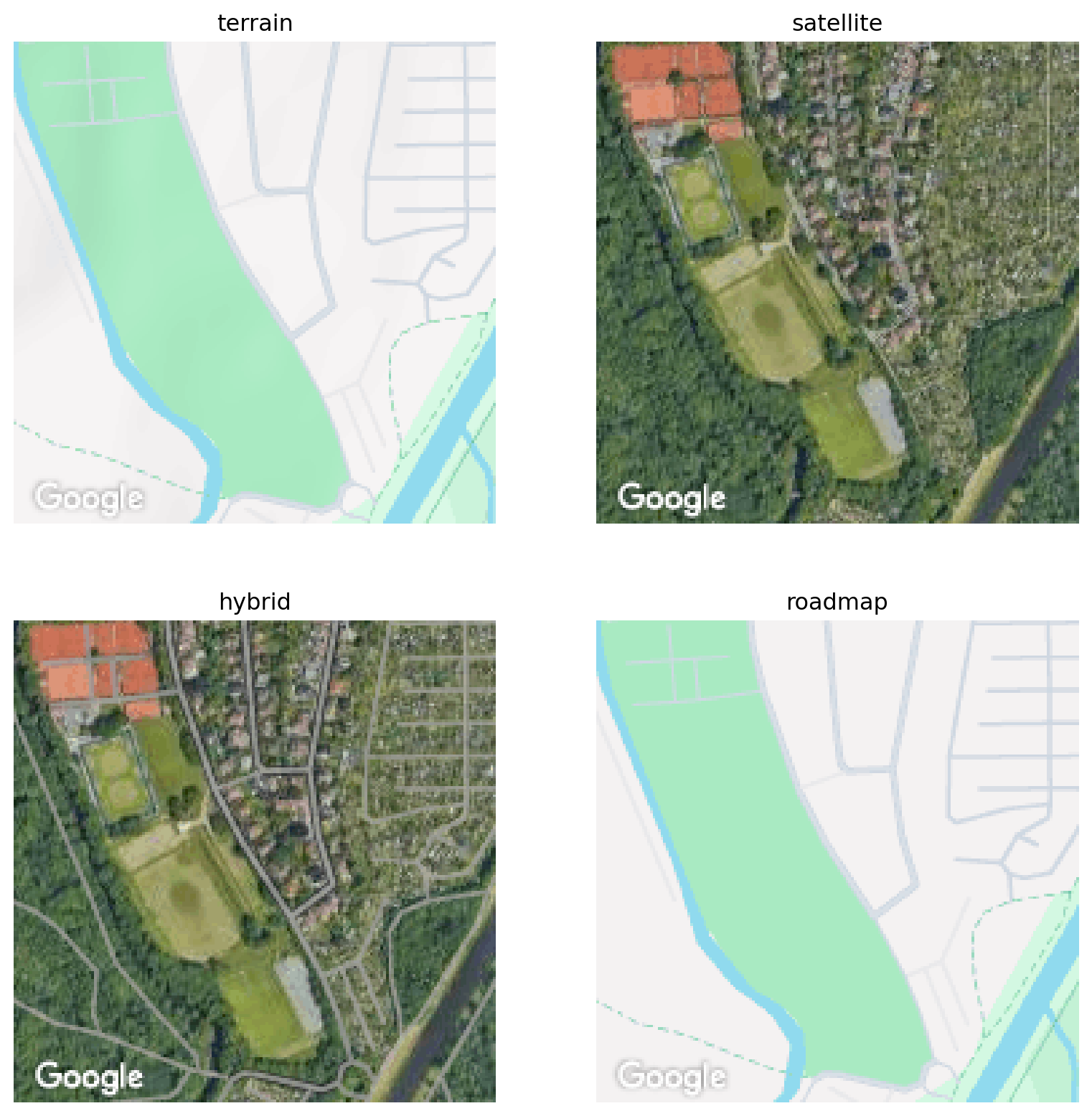
We choose an image size of 180x180 here, which leaves us room to crop out the google watermark at the bottom of the image, by applying a central crop of 150x150 pixels to the image. The zoom level is set to 15 and is chosen so that each image contains enough context for the classifier and for the labelling process to decide wether it belongs to an urban or a rural area. I went with the hybrid images because they contained the most information, and the highlighted streets and paths make it easier for me to label the images and decide to which class an image belongs. The resolution of the images is quite low, but I suspect that there is still enough information present in the image to work well in the classification task, while we'd like to keep the image size as small as possible. This is because the size of the images determines the input shape into our neural network, which in turn determines the number of parameters in the model. To keep the training time low and also care for the limited hardware resources, this is desirable.
For building the training data set, we go with a moderate size of 5000 map images, to start with. For the purpose of this classifier, it will be enough to incorporate map images from germany, since the classifier is intended to classify locations from my cycling data, which contains locations from germany, for the most part. So we're randomly sampling 5000 lat/lon coordinates from germany, with this little helper function, using a shapefile for germany, which gives us the boundaries of germany as a polygon:
def sample_german_locations(num_points: int, shapefile_path: str, ):
# sample random points as lat, lon coordinates within germany
germany_shape_df = gpd.read_file(shapefile_path).to_crs("EPSG:4326")
# total germany shape
germany_bound = germany_shape_df.geometry.union_all()
# get the boundary of germany
bounds_all = germany_bound.bounds
minx, miny, maxx, maxy = bounds_all
i = 0
points = []
while i < num_points:
    # generate random location coordinates
    x_t = np.random.uniform(minx, maxx)
    y_t = np.random.uniform(miny, maxy)
    if germany_bound.contains(Point(x_t, y_t)):
        i += 1
        points.append((x_t, y_t))
return points
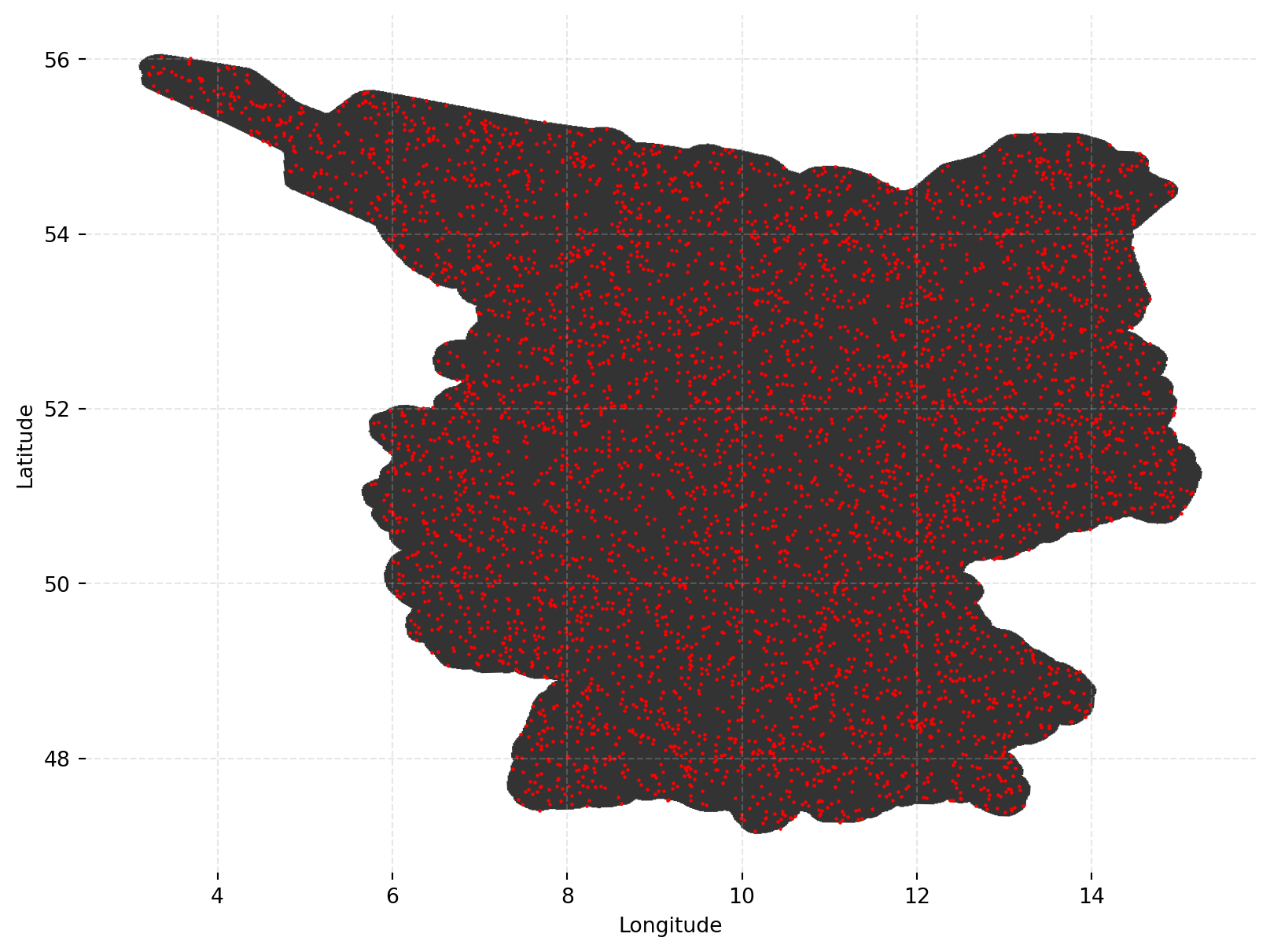
See the map below for the random locations of the 5000 map images we'll subsequently download from google maps.
We then use these coordinates as the central location to query the google API,
and we get 5000 images of 150x150 pixels after cropping, which we store on
disk as .npy files for the next step, which is annotating the
images wit the corresponding labels.
Annotating the Labels
In order to obtain the ground truth labels for the images, we use a simple script, which runs in a jupyter notebook. There is no need for fancy annotation tools here. Let's keep in mind here, how we intend to use the classifier later. We want the classifier to classify locations which are in the very center of the image, representing the location of the rider. So it's the central image location, which is crucial for the classification. The script, therefore displays each image one after the other with a little red dot in the center of the image to guide our annotation process. We use keys to do the labelling, where we need one key for 'rural', one key for 'urban', and a third one for images that are 'invalid'. This is because we sampled the images randomly, so there will be a portion of map images that are completely over lakes or inside a coal mine, for instance, which are regions that I'll never pass with my bike. See the code below for the core annotation function:
def label_images(imgs: list)->dict:

# imgs is a list of paths to the images

labels = {}
for idx, img in enumerate(imgs):
    arr = np.load(img)
    w, h, _ = arr.shape
    # plot red point in center as a reference point
    plt.plot(w // 2, h // 2, marker='o', color="red")
    plt.imshow(arr)
    plt.show()
    print("Choose 'q' if rural, or 'e' if urban, or 'w' if invalid:")
    x = "g"
    while x not in ['q', 'e', 'w']:
        x = input()
        if x == 'q':
            labels[img] = "rural"
            print("rural")
        elif x == 'e':
            labels[img] = "urban"
            print("urban")
        elif x == 'w':
            labels[img] = "invalid"
            print("invalid image")
        else:
            print("invalid input")
    clear_output(wait=False)

return labels
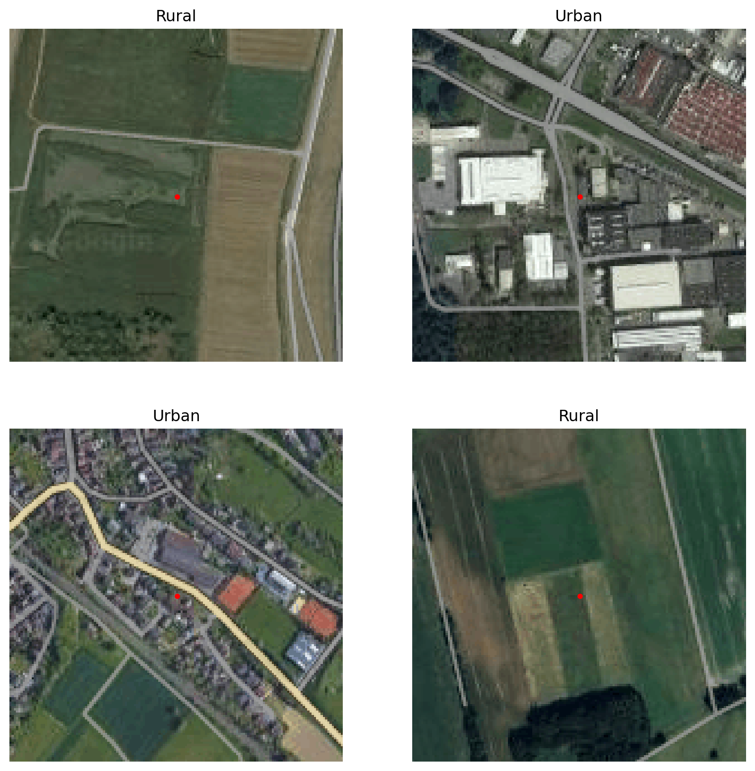
As you might expect, doing this for 5000 images is quite a tedious task. Another aspect to consider here is, that we sampled the image locations randomly. This means that we'll get far less images of urban areas, than of rural areas, because this is just the distribution of these areas in germany. This is crucial, because in binary classification tasks, we want to have a balanced data set, where one class isn't much more frequent than the other. Nevertheless I decided to go with 1.5 times more rural images than urban images, to have a bigger data set after all, since there were just 268 urban images in the 5000 samples. The whole dataset contains 832 images, which is really a small data set for neural network training, but since labelling these by hand is really no fun at all, we'll stick with this for now and make extensive use of data augmentation in the next step, to increase the size and diversity of the data set. We'll set the train/test ratio to 80/20, to get as much data as possible for training, since we have so few images. Certainly, this potentiall compromises the trust we may have in our validation metrics, but trade-off are neccessary here. See the figure below for a few sample images from the train and test data sets. The red dots, of cause, are not present in the images, they are just for referrencing the hypothetical riders position.
Train Samples
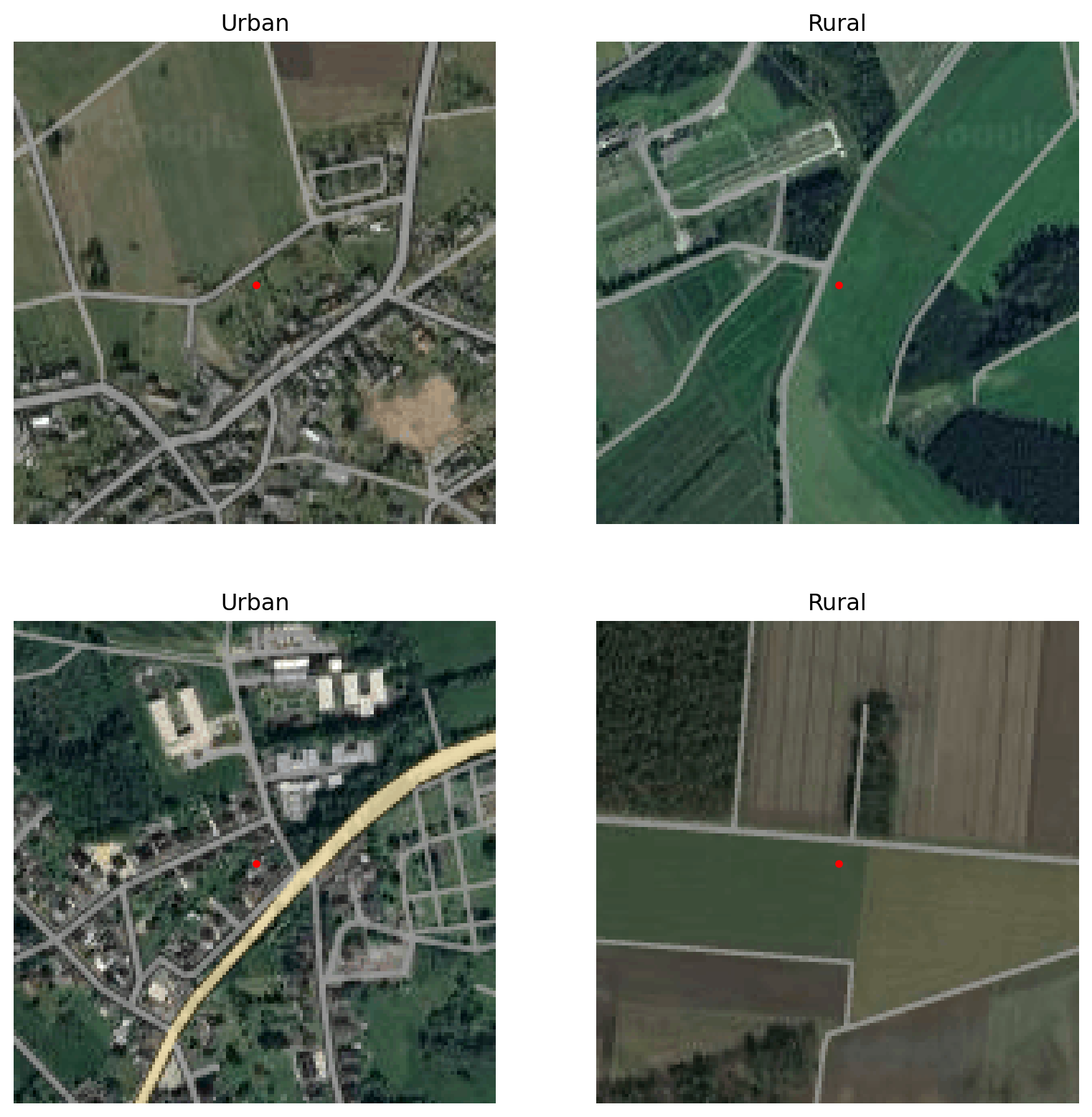
Test Samples
3. Model Architecture
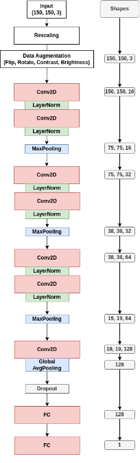
When choosing the right architecture for the classifier, we try to stick with the 'keep it simple, stupid' principle. I suspect that the classification problem at hand, really isn't too hard for neural networks to solve. But its obvious that our network should learn abstract features like edges and corners, since the streets and buildings in urban areas form regularities and patterns. A perfect job for a convolutional neural network (CNN). Since we like the neccessary computational resources to be moderate, we'll build a simple CNN with just a few layers. If we reach good enough performance with this there is no need to utilize bigger models like, for instance, models from the ResNet family. See the architecture in the figure for an overview of the model. As you can see, we implement the data augmentation directly in the model as one of the first entry layers. Here we randomly flip the image horizontally and vertically, rotate the image by a maximum of plus or minus 1 pi and apply random contrast and brightness changes to the image. This way we can increase the effective size of the data set and also make the model more robust to differences in the map images used for inference later, as these qualities of google maps images can vary quite a bit. For the convolutional layers we use a kernel size of 2 and relu activation functions. For the three Conv2D blocks we apply 16, 32 and 64 filters for the two subsequent Conv layers in each block. At the final layer of the model we obain the bare logits, which we'll pass to our Binary Crossentropy loss function, to get the final classification.
4. Model Training and Evaluation
Training
For the model training process, a new set of randomly sampled augmentations are applied by our augmentation layers every epoch. We train for 30 epochs with a batch size of 16 and save the best model according to the validation accuracy. The quasi standard Adam optimizer with a learning rate of 0.0001 is used. After the training we can observe the following training curves:
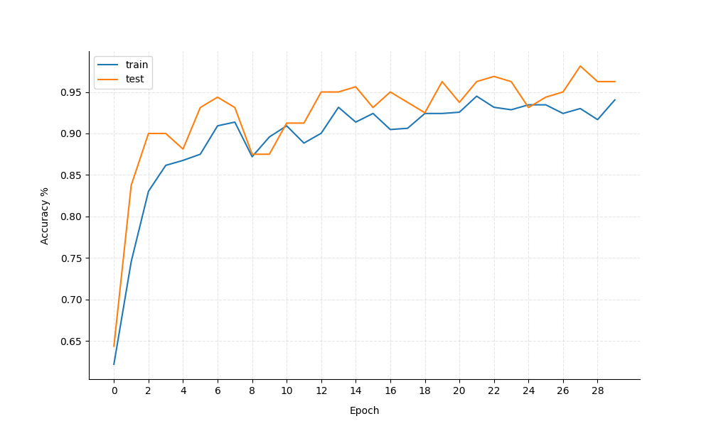
The model reaches a validation accuracy of 96.875 during training, which is decent for our task. The bumpy curves of the accuracies is most likely due to the small size of the data set and the random nature of the data augmentation. Let's look at some evaluation metrics to shed some more light on the model performance.
Evaluation
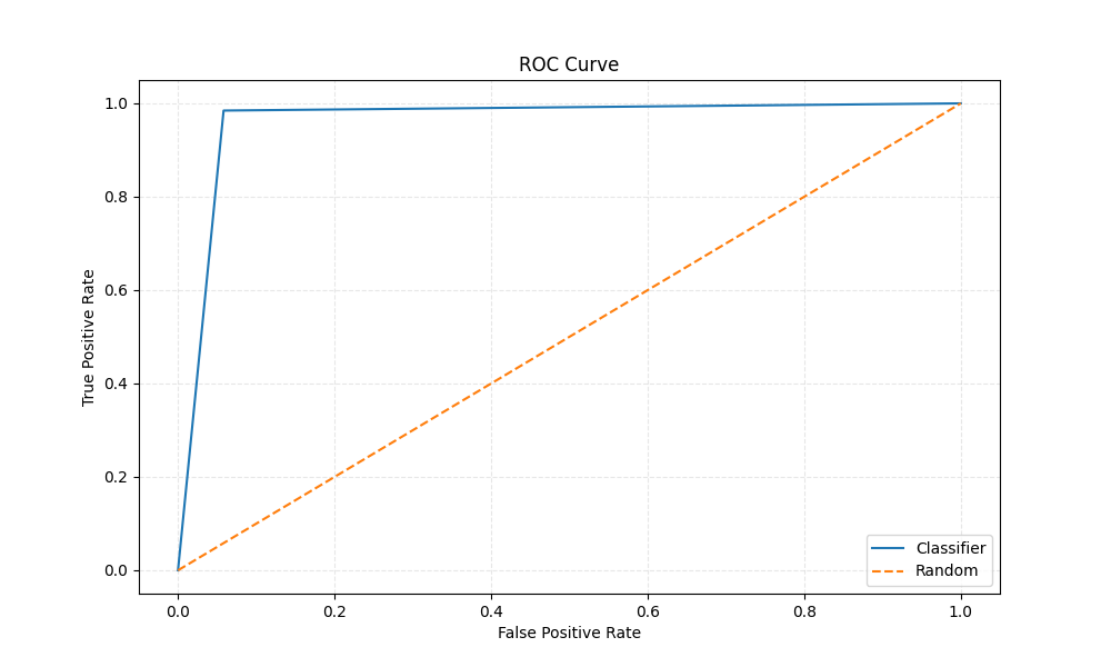
For the evaluation of the model, we'll look at the ROC curve, precision, recall and the f1-score, computed on the test set of the data. The ROC curve is a good indicator of the models performance, since it shows the trade-off between the true positive rate and the false positive rate. We find a roc-auc score of 0.9632.
The precision, recall and f1-score for the classifier are observed as follows:
| Precision | Recall | f1-score | |
| rural | 0.99 | 0.94 | 0.97 |
| urban | 0.91 | 0.98 | 0.95 |
As we can see, the classifier perfroms slightly better in correctly detecting urban areas than rural areas. The most common mistake the classifier makes is falsely predicting rural areas as urban, which is reflected in the corresponding precision value for urban and the corresponding recall value for rural. When labelling the images I suspected that the classifier will have problems when the central location is right at the edge of a town, where the urban and rural areas meet. This is because even for me it's hard to decide wether the location is urban or rural. So I'm sure with an not so consequent labelling, the classifier will have problems in these areas too. Lets look at some falsely as urban classified images from the test set:
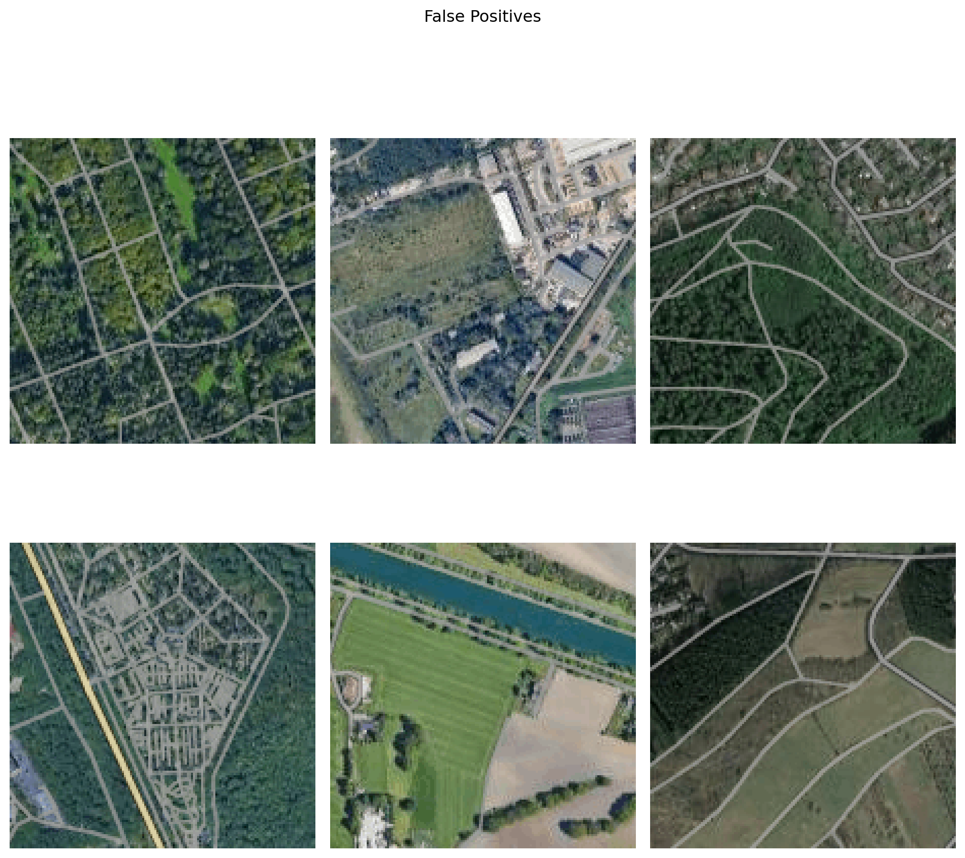
In the top middle and right we can see cases of beeing at the edge of a town, which is expected, to be hard for the classifier to classify correctly. Top and bottom left, we might assume that the structures we see there might have similarities with patterns we typically find in cities. The bottom middle and right missclassifications are a bit surprising, though. Probabely with more data and better label annotation, errors like that could be avoided.
Overall I'm happy with the result. With the reported performance it is possible to use this in my cycling data analysis project, to classify the riders locations without introducing too much bias. Sure there are many ways to improve the model, like using a bigger data set, better, more accurate labelling, more complex model architectures, or even using pre-trained models. But since this side-project is embedded within a bigger project, and time is a valuable resource I'll use it like that.It serves my goals well enough. Of cause this approach may be extended to classifying more relevant structures, like forests or mountains or even to classify the type of urban area, like residential, industrial or commercial areas. Maybe you have a use case for this and time and motivation to build uppon this approach.