Local Retrieval of OSM Tags
1. Introduction
For my cycling data analysis project, there is the neccessity to get information about certain attributes of roads. Usually one is cycling on different kinds of roads, streets, little paths, which all may have different attributes and which may all have thus a different influence on ones riding speed. The problem setup is as follows: I have a dataset of over 150.000 rows, for each row I have lon/lat coordinates. Based on these coordinates I want to know as much about the road, at each of the individual coordinates, as possible. This post is about how I approached this problem by using OpenStreetMap (OSM) data and how I implemented the retrieval of these information. The challenge here is the amount of data that has to be retrieved, as well as having control over the retrieval process and the quality of the data, since the data will be used in a machine learning application, where it is crucial to know your data. For this reasons we're not using any kind of web-based OSM API, or reverse geocoding API, but we'll solve this locally. One of the many good things that OSM brings to us is that it is information rich and that we can download datasets. Thus we have control over our whole processes. For me, as a OSM novice, this came with some unknown challenges, where I'll try to explain my approach here. Hopefully this will help anyone, who is facing similar tasks, and is just starting with the world of OSM data.
2. Why local OSM?
Surely, there is a whole ecosystem of geocoding services out there in the web (like GeoApify or Nominatim or Overpass). But for a hobby project like this, one doesn't want to pay quite a bit for services, or to be limited in the amount of requests, either by price or by usage policy. Don't get me wrong, there are cetrainly a lot of use cases where you can come away with free services, but if the amount of requests to solve your problem grows this becomes more and more infeasible. Also one is missing out on the opportunity to learn a lot of useful stuff. OSM provides an ever growing database of spatial information for the whole planet. Especially for data requests in Europe, OSM provides a lot of information. Check out this nice node density map: OSM Node Density. For my project I have to retrieve information for coordinates in Germany and and a bit around, so as the map suggests, OSM data is quite the ideal data source.
3. Data! Where, How?
Crazy enough, you really can download the OSM data of the whole world in one file, which is the Planet.osm. While this is not neccessary for my needs, thankfully there are providers of sub-region extracts like Geofabrik, where one can download the, regularly updated, data for a specific region in a single '.pbf' file, which is protocol buffer file, that stores the data in a quite compressed binary format. To get the data, we just download the Europe extract, which is abaut 29 GB in size. So we just do:
cd /path/to/your/data
wget https://download.geofabrik.de/europe-latest.osm.pbf
Little OSM stack
Let me briefly compile the tools for this task. In general, we're using Python 3.12 on a Ubuntu 24 system, with regular data wrangling and data science tools already there, like: pandas, numpy, scikit-learn and matplotlib. We'll further need:
| Tool | Function |
| osmium | command line tool for OSM data processing |
| pbf2sqlite | simply writes contents of .pbf file into a local SQLite DB |
| SpatiaLite | Extension to SQLite for Spatial SQL capabilities |
| Geopandas | Nice geospatial functionalities, depends on shapely, which we need too |
The OSM data model and .pbf structure
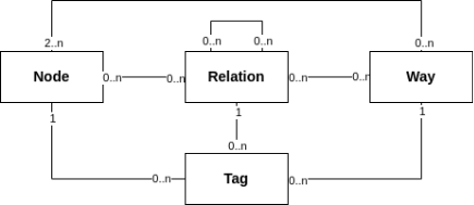
To understand the ramainder of the article, it is neccessary to have a glimpse about the OSM data model. There are three types of objects, which are nodes, ways and relations. Nodes are the basic elements of the OSM data model, and they have lon/lat coordinates as attributes. Ways are ordered lists of nodes, which represent linear features like streets or rivers, they can have multiple tags that describe them. Relations are ordered lists of nodes, ways or other relations, which are used to describe more complex structures like routes or boundaries. In this project, we're mainly interested in the tags of the ways, so we won't deal with relations at all. The .pbf files are sequentially structured, which means that if you're iterating over the whole file, your iterator sees first all nodes, then all ways and then all relations. There are python bindings for osmium, which are provided in the pyosmium library. We could use this library to read the pbf-file we obtained from Geofabrik, but this will be really, really slow. We have to crunch some numbers to get the closest way to each of our coordinates, and iterating over the pbf file would mean to manage complex data structures to keep track of seen nodes and ways, and iterate over the whole file over and over again. This is not a feasible solution for this amount of coordinates (recall, over 150.000) we have, since iterating over the whole file with osmium takes a few minutes on my machine. We'll have to come up with a faster solution.
4. Querying Quickly
The solution to this problem is using a DBMS to hold the data and manage the queries. For small projects like this, of cause, SQLite is the perfect candidate, since we will write the database once, then just do reads, which SQLite can also handle with multiple reading DB connections. So the strategy is as follows:
- on the europe extract, use osmium to extract the ROI to get a smaller extract
- convert the data from the extract extract to a SQLite database
- enable the SpatiaLite extension for the DB and build a spatial index
- come up with a multiprocessed querying strategy, to retrieve the tags of interest
Let's go through these steps one by one. First we're retrieving the maximum and minimum lon/lat coordinates from our pandas data frame. Check out my post about my cycling data analysis, if you want to know more about this data. We extend these coordinates by a little margin, to be sure, that we really covered the whole region of interest.
# python3
# get the min and max lon/lat coordinates from df
min_lat = df["lat"].min()
max_lat = df["lat"].max()
min_lon = df["lon"].min()
max_lon = df["lon"].max()

# add an epsilon to the min/max coordinates as a buffer
eps = 0.1
min_lat -= eps
max_lat += eps
min_lon -= eps
max_lon += eps
Next, we'll use osmium to extract the region of interest from the europe extract, like so:
osmium extract -b $maxlon,$maxlat,$minlon,$minlat europe-latest.osm.pbf -o cycling_df_extract_roi.pbf
And use pbf2sqlite to write the contents of the extract to a SQLite database. This will take a while, depending on the size of your extracts, in my case the extract was about 5GB in size, which resulted in a 11GB database file.
cd /path/to/pbf2sqlite/
python3 pbf2sqlite.py /path/to/osm_cycling.db /path/to/cycling_df_extract_roi.pbf
Once the data base is built, we can enable the SpatiaLite extension and build a spatial index. Keep in mind, that the index will take a lot of additional disk space, as it has to be built upon possibly billions of lon/lat coordinates from the nodes.
# add spatialite index
with sqlite3.connect("/path/to/osm_cycling.db") as conn:
conn.enable_load_extension(True)
conn.execute('SELECT load_extension("mod_spatialite")')
conn.execute('SELECT InitSpatialMetaData(1);')
conn.execute(
    "SELECT AddGeometryColumn('nodes', 'point_geom', 4326, 'POINT', 2);"
)
conn.execute("UPDATE nodes SET point_geom = MakePoint(lon, lat, 4326);")
conn.execute(
    'SELECT CreateSpatialIndex("nodes", "point_geom");'
)
conn.commit()
Writing out the DB Queries
Let's recall, what we want to achieve: for a given lon/lat coordinate, we like to find the closest way in the OSM data, and retrieve the set of tags for this way. One of the most common tags for ways, we're after, is the 'highway' tag. For extensive information on OSM tags, see taginfo. So we narrow down our task as finding the closest way with a highway tag, since there can be close ways which are not streets or paths in our sense. First let me show how we use the spatial index. We have to compute a bounding box around our coordinate of interest, first. Then we use the coordinates associated with the bounding box to make our query. To compute the bounding box, we use a little helper function, again using an epsilon as an offset:
def get_bbox(coordinates: tuple, eps: float = 0.001)->dict:
# coordinates are ordered lon, lat
bbox = {
"bbox_minx": coordinates[0] - eps,
"bbox_maxx": coordinates[0] + eps,
"bbox_miny": coordinates[1] - eps,
"bbox_maxy": coordinates[1] + eps
}
return bbox
To get all the nodes in the bounding box we query the DB like this:
c.execute(
f"""
SELECT node_id
FROM nodes
WHERE
    nodes.rowid IN (
        SELECT pkid
        FROM idx_nodes_point_geom
        WHERE xmin > :bbox_minx
            AND xmax < :bbox_maxx
            AND ymin > :bbox_miny
            AND ymax < :bbox_maxy
    );
""",
bbox
)
The table nodes here holds all the nodes in the OSM
dataset, with their corresponding node_id, lat and lon values! With the
node ids we can find the way, which the node is part of. We then have
to figure out which of the ways is closest to our query coordinate. The procedure is as follows:
- query for the coordinate and join with the way_nodes table, we get all the distinct ways which are referencing the nodes in the bounding box
- for each of the way ids, query all the node_ids and their corresponding lon/lat coordinates
- for the coordinates of each way, construct a shapely linestring and store them in a geopandas data frame
- for all the linestrings, compute the shortest distance to the query coordinate
- order the ways by the just computed distances
- iterate over the sorted ways and query the tags for these ways
- stop at the first way with a 'highway' tag and return this as result
The crucial part here is to compute the distances in meters between the query coordinate and the linestrings. We use geopandas for this which provides a handy method. We just have to wrangle a bit with geopandas data frames:
def get_dists_to_point(pnt: tuple, lines: list)->gpd.GeoSeries:
# both must be lon/lat
linestrings = [LineString([(k[0], k[1]) for k in x]) for x in lines]
point = Point(pnt)
gdf_point = gpd.GeoSeries([point], crs="EPSG:4326")
gdf_point = gdf_point.to_crs(gdf_point.estimate_utm_crs())
gdf_lines = gpd.GeoDataFrame(geometry=linestrings, crs="EPSG:4326").to_crs(gdf_point.crs)
distances = gdf_lines.distance(gdf_point.iloc[0])
return distances
As this is still quite a bit work to do for each of the over 150.000 coordinates,
it's certainly a good idea to parallelize this task. For this we cast our querying
procedure into a python function and use the multiprocessing library to process the
queries concurrently.
# query_db_by_coord is our db querying function here

# store the candidate coordinate pairs in a list
coordinate_units = df[["lon", "lat"]].values.tolist()

# use a pool to spawn the process workers
with Pool(16) as p:
results = p.map(query_db_by_coord, coordinate_units)
In my case, this still took around 1 and a half hours to complete, but certainly it's worth the effort.
Inspecting the Results
Let's have a look what we found in the OSM extract. I also stored the distances of the ways which are considered the closest. We can plot them to see if we found ways which are too far off our query coordinates to be considered a valid result.
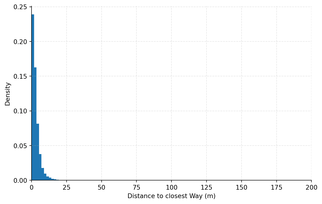
This looks quite promising, since we seem to have a negligible amount of ways which are far off the query coordinate. Now let's have a look what kind of tags we found for the ways. We can easily plot the 10 most common tags and their coverage in percent:
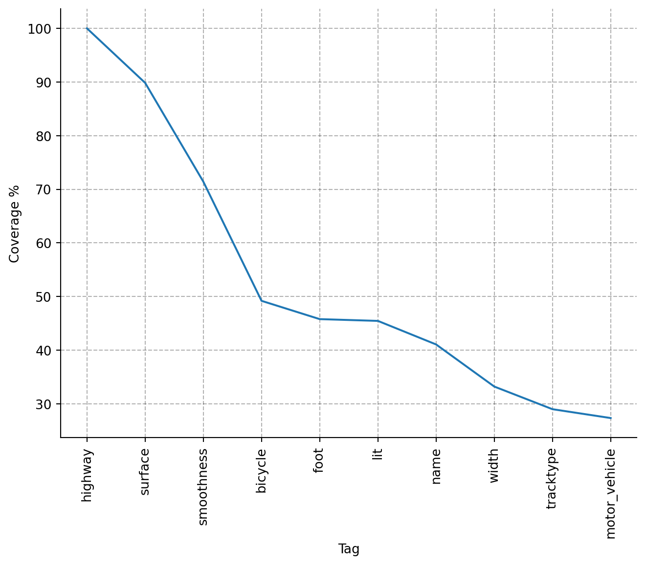
For my cycling data project I decided to take just the three most common tags, as they have decent coverage in the retrieved data. The missing values will be imputed later. The retrieved tags are key-value-pairs, and I have to do some cleaning and clustering of all the possible values for each tag, to use this data in my analysis, but this isn't too much work. All in all this was a fun side project, which teached me a bit about OSM data and how to handle it. Right now, I'm imagening all the interesting features for any kind of spatial analysis one could engineer from this data. I'm a bit hyped, I must say. Probabely you're too. :)